1. Sourced a real climate dataset
I sourced a real, science-backed dataset instead of reusing healthcare_dba from Project 1, since the whole point of this project is to start with a fresh, intentionally unoptimized "before" state I can diagnose and fix in later phases. I chose NOAA's Global Historical Climatology Network Daily (GHCN-Daily) — the same dataset used in peer-reviewed climate research, distributed under a CC0 public domain license.
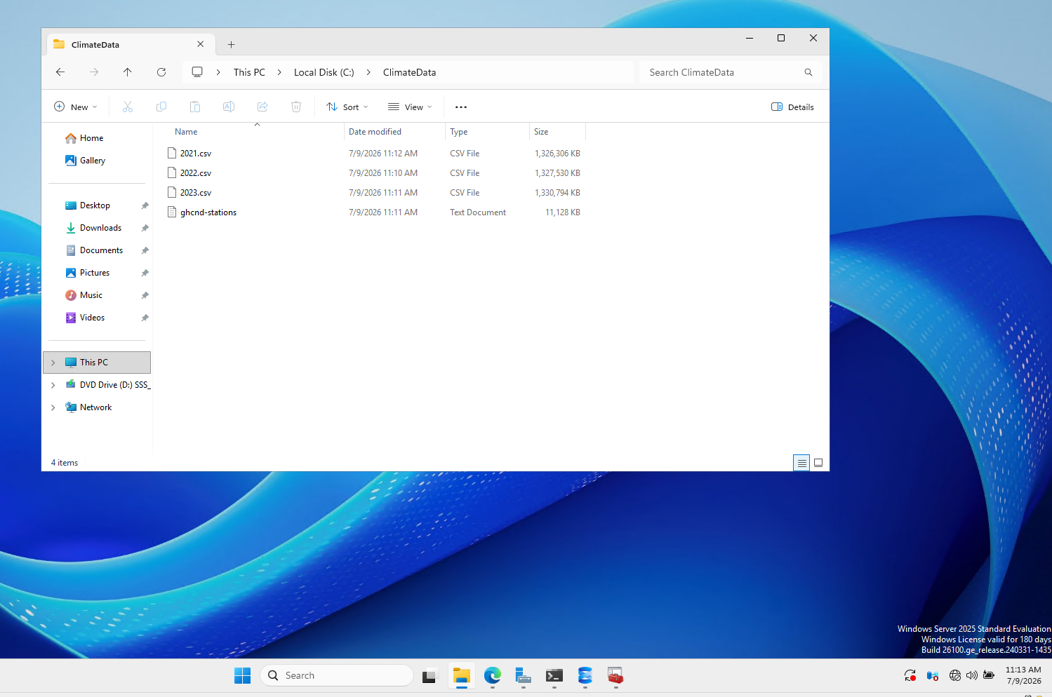
I downloaded three years of daily observation data (2021.csv, 2022.csv, 2023.csv, ~3.8GB combined) plus the station metadata file (ghcnd-stations.txt, ~10.9MB) directly from NOAA's public S3 bucket.
csv/2023.csv) returned a NoSuchKey error. NOAA had restructured their bucket prefixes, and the correct path needed an extra by_year/ segment (csv/by_year/2023.csv). I documented this rather than quietly routing around it, since it's exactly the kind of real-world gotcha worth keeping visible.2. Moved the raw data into the VM
Since SQLDBA-Primary is a separate Hyper-V VM, I needed a way to get these files onto it. I enabled Hyper-V's Guest Services integration service, which let me copy files directly between my host and the VM console — no shared network folder needed for this one-time transfer. I moved all four files into C:\ClimateData\ inside the VM.
3. Created the new database
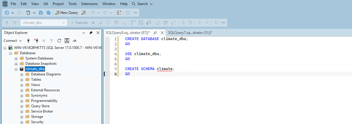
I created a new database, climate_dba, alongside the existing healthcare_dba, deliberately kept separate rather than replacing it.
4. Designed the schema — deliberately unoptimized
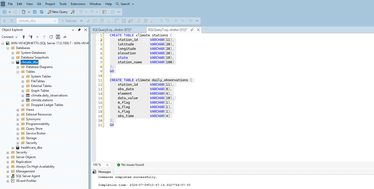
I created a dedicated climate schema containing two tables:
- climate.stations — station_id, latitude, longitude, elevation, state, station_name (all VARCHAR, no keys or indexes)
- climate.daily_observations — station_id, obs_date, element, data_value, m_flag, q_flag, s_flag, obs_time (all VARCHAR, no keys or indexes)
This is deliberately naive: no primary keys, no foreign key relationship between the two tables, no indexes on the columns I'd obviously query on (station_id, obs_date), and dates/numbers stored as text instead of proper types. This matches how a rushed first pass at this data would actually look, and gives me a real "before" state to improve in Phase 4.
5. Loaded the station metadata
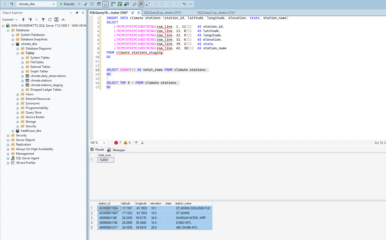
ghcnd-stations.txt is a fixed-width file, so I loaded it into a staging table (climate.stations_staging) as raw text lines first, then parsed it into climate.stations using SUBSTRING based on the documented column positions.
BULK INSERT to actually read the file correctly took two failed attempts. I initially assumed the file used a standard Windows \r\n line ending and specified ROWTERMINATOR = '\r\n', which failed. Checking the raw bytes showed the file actually uses bare Unix-style line feeds (0x0A). The real fix was realizing T-SQL doesn't interpret '\n' as an escape sequence — it reads it as two literal characters, not a newline. Using the hex literal ROWTERMINATOR = '0x0a' fixed it immediately.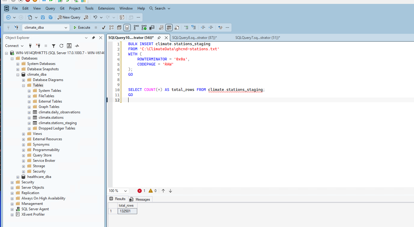
After parsing into the real table, I confirmed 132,501 rows with realistic, correctly-split data.
6. Bulk-loaded three years of observations
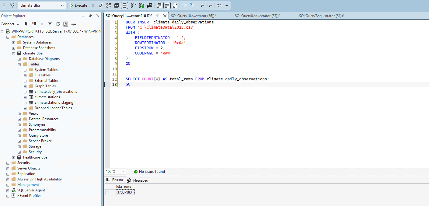
Loading the three yearly observation CSVs was more straightforward once I knew about the line-ending issue — same 0x0a row terminator, comma field terminator, and FIRSTROW = 2 to skip a header row I discovered these files actually have.
2023 alone loaded 37,907,983 rows:
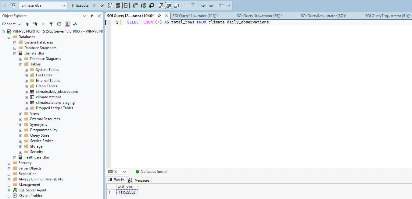
All three years combined loaded 113,522,932 rows total:
7. Ran baseline diagnostics on the unindexed schema
With the data loaded, I ran two realistic queries against the schema as-is to establish a documented "before" state.
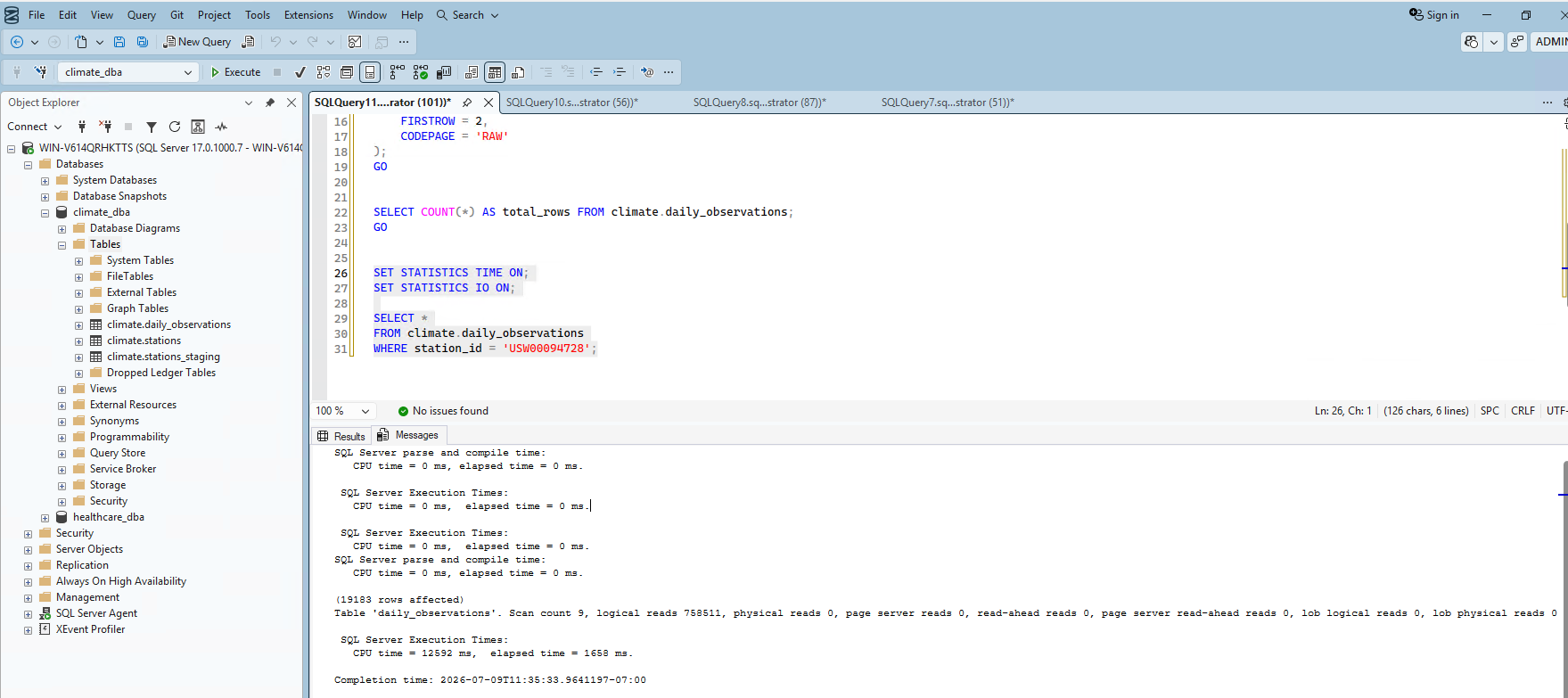
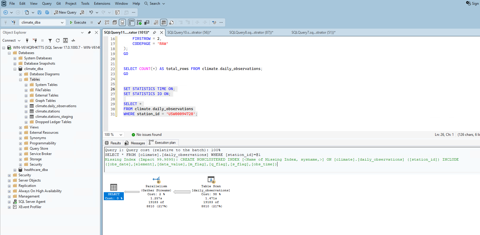
Query 1 — filter by station_id:
SELECT * FROM climate.daily_observations WHERE station_id = 'USW00094728';- 19,183 rows returned
- 758,511 logical reads, scan count 9 (parallel table scan)
- 1.658 seconds elapsed
- SQL Server's own missing-index recommendation: nonclustered index on
station_id, estimated 99.5% impact
Query 2 — filter by date range:
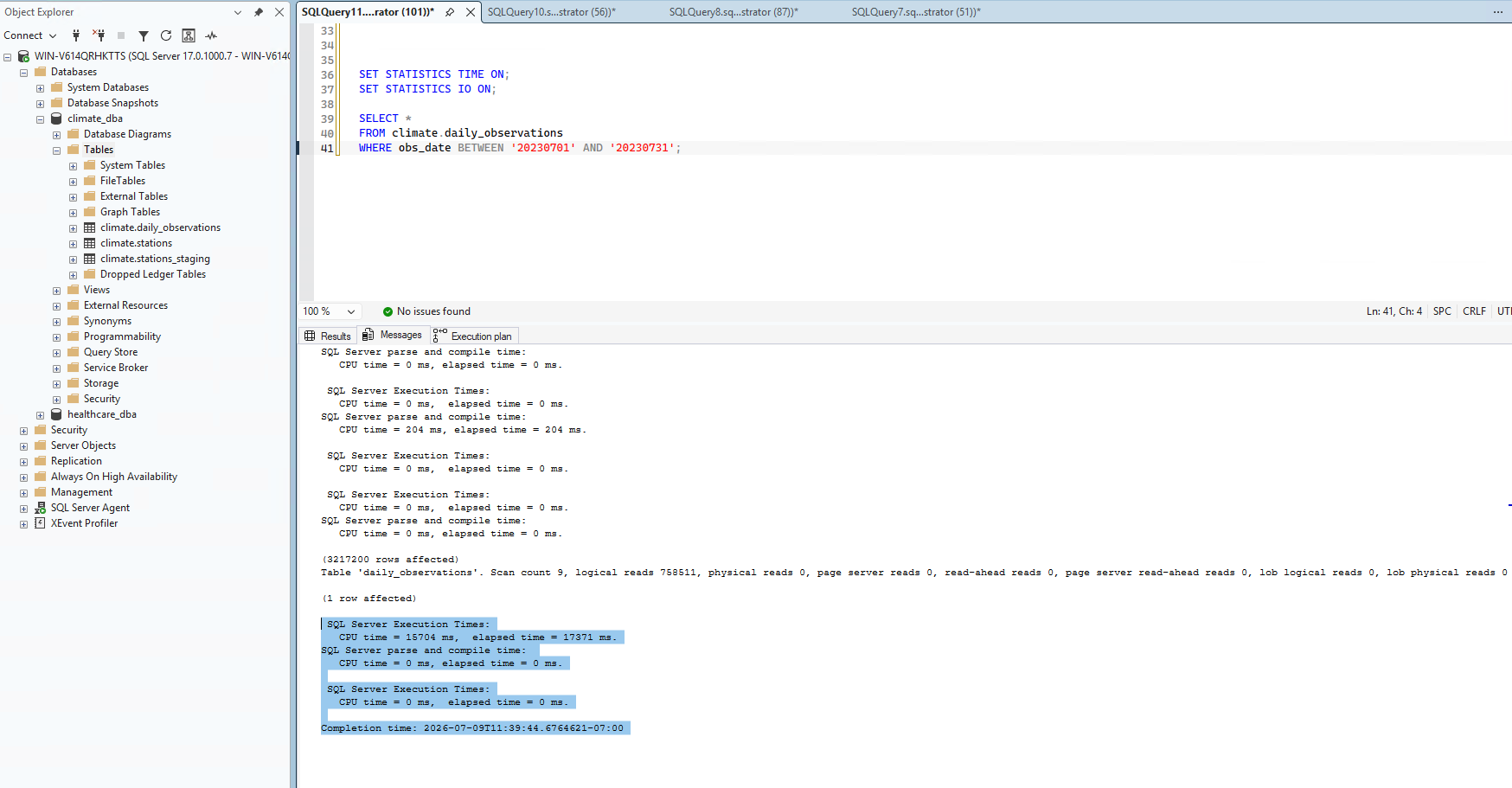
SELECT * FROM climate.daily_observations WHERE obs_date BETWEEN '20230701' AND '20230731';- 3,217,200 rows returned
- 758,511 logical reads, scan count 9 — identical I/O cost to Query 1, since both force a full scan of the same table regardless of which column is filtered
- 17.371 seconds elapsed — notably slower than Query 1, which I attribute to the much larger result set being returned to the client rather than a difference in scan cost
- SQL Server's missing-index recommendation here: nonclustered index on
obs_date, estimated 68.3% impact
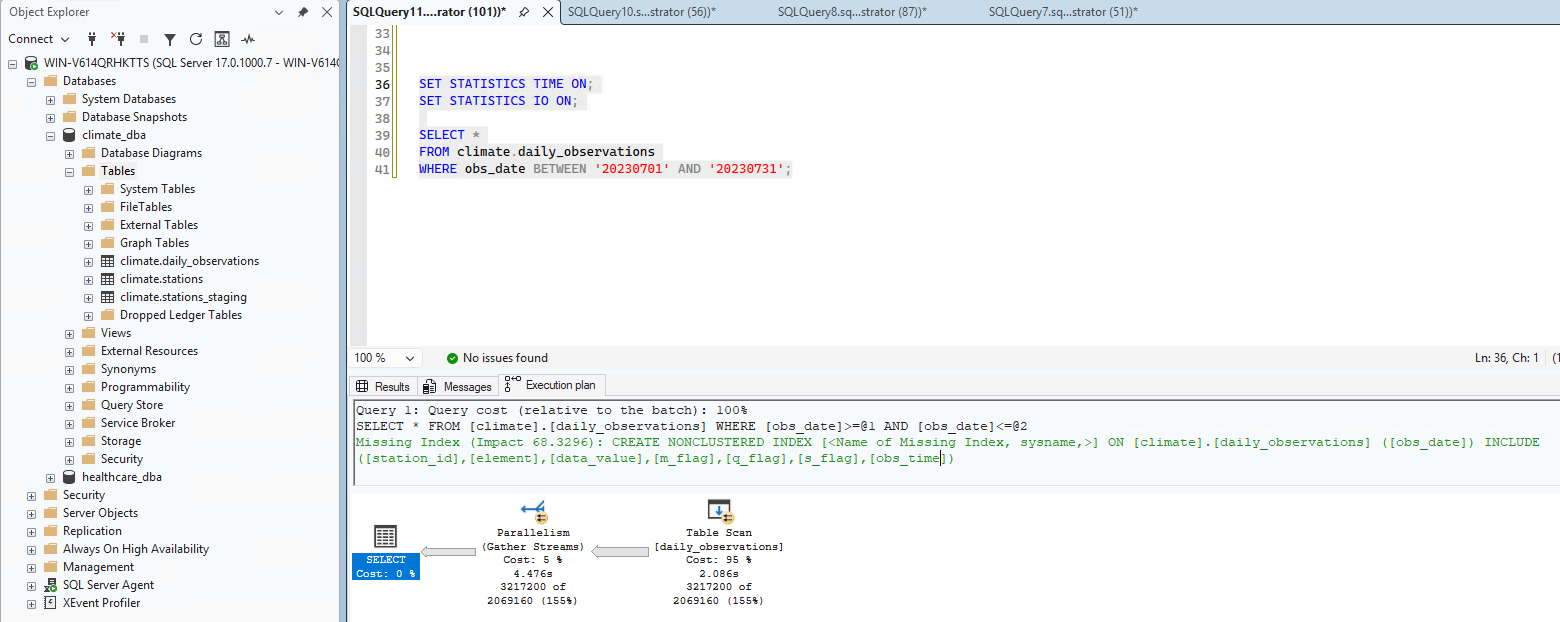
Both execution plans confirm a full Table Scan with Parallelism, and both show SQL Server's row estimates were significantly off from actual row counts (155–217%) — a direct consequence of having no statistics maintenance or proper indexing on this table yet.
What's Next
This gives me two real, reproducible baseline numbers — and two competing missing-index recommendations (one on station_id, one on obs_date) — that I'll come back to in Phase 4 to design a real indexing strategy and measure genuine improvement, rather than just applying whatever SQL Server suggests without thinking it through.